Fast evaluation of Fourier series at arbitrary points
This is a simple demo of using type 2 NUFFTs to evaluate a given 1D and then 2D Fourier series rapidly (close to optimal scaling) at arbitrary points. For conciseness of code, we use the MATLAB interface. The series we use are vaguely boring random ones relating to Gaussian random fields—please insert Fourier series coefficient vectors you care about.
1D Fourier series
Let our periodic domain be \([0,L)\), so that we get to see how to rescale from the fixed period of \(2\pi\) in FINUFFT. We set up a random Fourier series with Gaussian decaying coefficients (this in fact is a sample from a stationary Gaussian random field, or Gaussian process with covariance kernel itself a periodized Gaussian):
L = 10;             % period
kmax = 500;         % bandlimit
k = -kmax:kmax-1;   % freq indices (negative up through positive mode ordering)
N = 2*kmax;         % # modes
rng(0);             % make some convenient Fourier coefficients...
fk = randn(N,1)+1i*randn(N,1);       % iid random complex data, column vec
k0 = 100;           % a freq scale parameter
fk = fk .* exp(-(k/k0).^2).';        % scale the amplitudes, kills high freqs
Now we use a 1D type 2 to evaluate this series at a large number of points very quickly:
M = 1e6; x = L*rand(1,M);        % make random target points in [0,L)
tol = 1e-12;
x_scaled = x * (2*pi/L);         % don't forget to scale to 2pi-periodic!
tic; c = finufft1d2(x_scaled,+1,tol,fk); toc   % evaluate Fourier series at x
Elapsed time is 0.026038 seconds.
Compare this to a naive calculation (which serves to remind us exactly what sum FINUFFT approximates):
tic; cn = 0*c; for m=k, cn = cn + fk(m+N/2+1)*exp(1i*m*x_scaled.'); end, toc
norm(c-cn,inf)
Elapsed time is 11.679265 seconds.
ans =
      1.76508266507874e-11
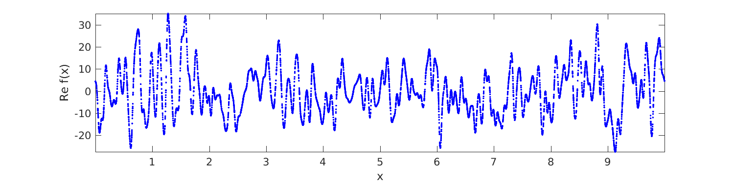
Thus, with only \(10^3\) modes, FINUFFT is 500 times faster than naive multithreaded summation. (Naive summation with reversed loop order is even worse, taking 29 seconds.) We plot \(1\%\) of the resulting values and get the smooth but randomly-sampled graph below:
Mp = 1e4;               % how many pts to plot
jplot = 1:Mp;           % indices to plot
plot(x(jplot),real(c(jplot)),'b.'); axis tight; xlabel('x'); ylabel('Re f(x)');
See the full code tutorial/serieseval1d.m which also shows how to evaluate the same series on a uniform grid via the plain FFT.
2D Fourier series
Since we already know how to rescale to periodicity \(L\), let’s revert to the natural period and work in the square \([0,2\pi)^2\). We create a random 2D Fourier series, which happens to be for a Gaussian random field with (doubly periodized) isotropic Matérn kernel of arbitrary power:
kmax = 500;                   % bandlimit per dim
k = -kmax:kmax-1;             % freq indices in each dim
N1 = 2*kmax; N2 = N1;         % # modes in each dim
[k1 k2] = ndgrid(k,k);        % grid of freq indices
rng(0); fk =  randn(N1,N2)+1i*randn(N1,N2);         % iid random complex modes
k0 = 30;                     % freq scale parameter
alpha = 3.7;                 % power; alpha>2 to converge in L^2
fk = fk .* ((k1.^2+k2.^2)/k0^2 + 1).^(-alpha/2);    % sqrt of spectral density
We then simply call a 2D type 2 to evaluate this double series at whatever target points you like:
M = 1e6; x = 2*pi*rand(1,M); y = 2*pi*rand(1,M);   % random targets in square
tol = 1e-9;
tic; c = finufft2d2(x,y,+1,tol,fk); toc   % evaluate Fourier series at (x,y)'s
Elapsed time is 0.092743 seconds.
1 million modes to 1 million points in 92 milliseconds on a laptop is decent. We check the math (using a relative error measure) at just one (generic) point:
j = 1;                        % do math check on 1st target...
c1 = sum(sum(fk.*exp(1i*(k1*x(j)+k2*y(j)))));
abs(c1-c(j)) / norm(c,inf)
ans =
      2.30520830208365e-10
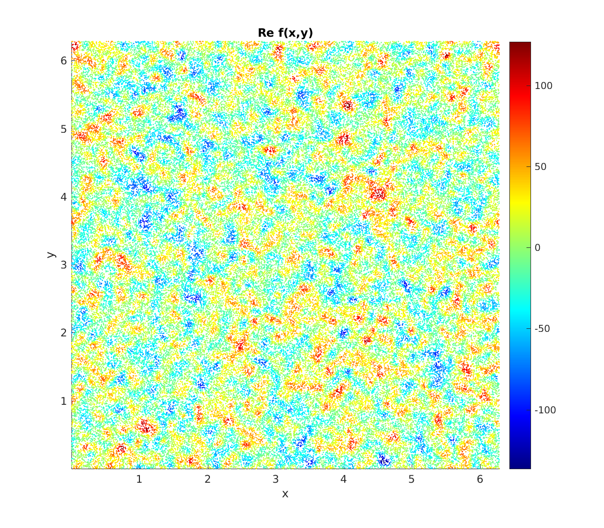
Finally we use a colored scatter plot to show the first \(10\%\) of the points in the square, and see samples of the underlying random field (reminiscent of WMAP microwave background data):
jplot = 1:1e5;           % indices to plot
scatter(x(jplot),y(jplot),1.0,real(c(jplot)),'filled'); axis tight equal
xlabel('x'); ylabel('y'); colorbar; title('Re f(x,y)');
See the full code tutorial/serieseval2d.m.