Efficient evaluation of (continuous) Fourier transforms¶

Say you want to evaluate the continous (as opposed to discrete) Fourier transform (FT) of a given function, but you do not know the analytic formula for the FT. You need a numerical method. It is common to assume that the FFT is the right tool to do this, but this rarely so …unless you are content with very poor accuracy! The reason is that the FFT applies only to equispaced data samples, which enforces the use of \(N\) equispaced nodes in any quadrature scheme for the Fourier integral. Thus, unless you apply endpoint weight corrections (which are available only in 1D, and stable only up to around 8th order; see references at the bottom of this page), you are generally stuck with 1st or 2nd order (the standard trapezoid rule) convergence with respect to \(N\). And there are many situations where a FFT-based scheme would be even worse: this includes nonsmooth or singular functions (which demand custom quadrature rules even in 1D), smooth functions with varying scales (demanding adaptive quadrature for efficiency), and possibly nonsmooth functions on complicated domains in higher dimensions.

Here we show that the NUFFT is often the right tool for efficient and accurate Fourier tranform evaluation, since it allows the user to apply their favorite quadrature scheme as appropriate for whatever nasty function they desire. As long as \(N\) is bigger than around 10, the NUFFT becomes more efficient than direct evaluation of exponential sums; as we know, most quadrature rules, especially in 2D or 3D, involve many more points than this.

1D FTs evaluated at arbitrary frequencies¶

Given a function \(f\), we’ll need a single quadrature scheme with nodes \(x_j\) and weights \(w_j\), \(j=1,\dots, N\), that allows accurate approximation of its Fourier integral

(1)¶\[\hat{f}(k) = \int f(x) e^{ikx} dx \approx \sum_{j=1}^N f(x_j) e^{ikx_j} w_j\]

for all “target” frequencies \(k\) in some domain of interest. You can apply the below to any \(f\) for which you have such a rule.

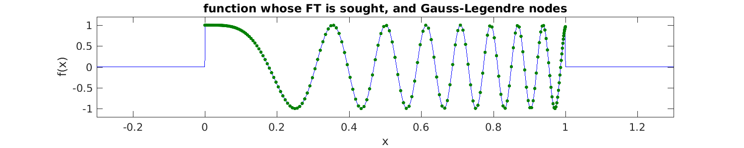
For simplicity let’s take \(f\) a smooth (somewhat oscillatory) function on \((a,b)\), choose a million random frequency targets out to some kmax, then pick Gauss-Legendre quadrature for \((a,b)\):

a=0; b=1;                     % interval
f = @(x) cos(50*x.^2);        % our smooth function defined on (a,b), zero elsewhere
M = 1e6;                      % # targets we want to compute the FT at
kmax = 500;
k = kmax * (2*rand(1,M)-1);   % desired target frequencies
N = 200;                      % how many quadrature nodes
[xj,wj] = lgwt(N,a,b);        % quadrature rule for smooth funcs on (a,b)

Below is \(f\) with the 200-node rule overlayed on it. You’ll notice that the rule seems to be excessively fine (over-resolving \(f(x)\)), but that’s because it actually needs to be able to resolve \(f(x) e^{ikx}\) for all of our \(k\) values:

Notice (1) is simply a type 3 NUFFT with strengths \(c_j = f(x_j) w_j\), so we evaluate it by calling FINUFFT (this takes 0.1 sec) then plot the resulting FT at its target \(k\) points:

tol = 1e-10;
fhat = finufft1d3(xj, f(xj).*wj, +1, tol, k);
plot(k, [real(fhat),imag(fhat)], '.');

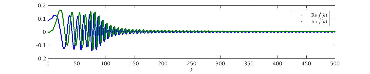
This looks like a continuous curve, but is actually (half a) million discrete points. Notice that because \(f\) was discontinuous on \(\mathbb{R}\), \(\hat{f}(k)\) decays slowly like \(|k|^{-1}\). How do we know to trust the answer? A convergence study in N shows that 200 nodes was indeed enough to reduce the quadrature error to below the \(10^{-10}\) NUFFT tolerance:

Ns = 100:10:220;             % N values to check convergence
for i=1:numel(Ns), N=Ns(i);
  [xj,wj] = lgwt(N,a,b);     % N-node quadrature scheme for smooth funcs on (a,b)
  fhats{i} = finufft1d3(xj, f(xj).*wj, +1, tol, k);
end
f0 = norm(fhats{end},inf);   % compute rel sup norm of fhat vs highest-N case
for i=1:numel(Ns)-1, errsup(i) = norm(fhats{i}-fhats{end},inf)/f0; end
semilogy(Ns(1:end-1),errsup,'+-');

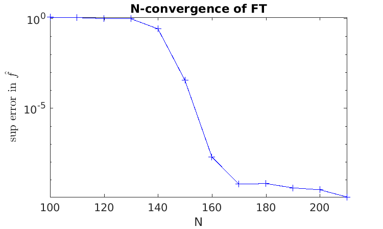
Remember: always do a convergence study! We see rapid spectral convergence as the quadrature rule resolves the oscillations in \(e^{ikx}\) at \(|k|=k_\text{max}\). See tutorial/contft1d.m for the full code.

Note

If you cared about only a few very high \(k\) values, numerical steepest descent applied at the endpoints \(a\) and \(b\) would eventually beat the above.

Faster FTs when frequencies lie on a grid¶

When the target frequencies lie on a uniform grid, the above type 3 NUFFT can be replaced by a type 1, which is faster, by a simple rescaling. Say that we replace the random targets in the above example by this uniform grid with spacing dk:

dk = 2*kmax/M;              % spacing of target k grid
k = dk * (-M/2:(M/2-1));    % a particular uniform M-grid of this spacing

Reusing our quadrature xj, wj from above, we wish to stretch the frequency grid from spacing dk to have unit spacing, which is the integer (Fourier mode) grid implied by (1), the definition of the type 1. This is equivalent to squeezing the inputs \(x_j\) by the same factor, which we do as we send them in:

cj = f(xj).*wj;             % strengths (same as before)
fhat = finufft1d1(dk*xj, cj, +1, tol, M);   % type 1, requesting M modes

This took only 0.05 sec, around twice as fast as before. We must check it is giving what we want:

fhat3 = finufft1d3(xj, cj, +1, tol, k);     % old type 3 method
norm(fhat-fhat3,inf)

which reports around 3e-11, so it worked. Note the specific offset of the k grid matched that of the Fourier mode indices; if you want a different offset, you will have to shift (by it to this specific offset, then post-multiply fhat with a corresponding phase.

1D FTs of singular functions¶

The above \(f\) was merely discontinuous. But you can now go further and easily replace \((x_j,w_j)\) by a rule that is accurate for a function with known singularities. Eg, say \(f(x) = x^{-1/2}g(x)\) where \(g\) is smooth on \([0,1]\), then the change of variable \(x=y^2\) means that \(\int_0^1 f(x) dx = \int_0^1 2y f(y) dy\), the latter having a smooth integrand to which plain Gauss-Legendre can be applied, giving a new rule \(x'_j = x_j^2\) and \(w'_j = 2x_j w_j\). Notice how this bypassed the pain of building a \((\alpha=0,\beta=-1/2)\) Gauss-Jacobi quadrature!

Let’s try out this new rule on a suitably singular function, keeping other aspects the same as the above type 1 method:

f = @(x) cos(50*x.^2)./sqrt(x);    % singular function defined on (0,1), zero elsewhere
Ns = 180:20:240;                   % N values to check convergence
for i=1:numel(Ns), N=Ns(i);
  [xj,wj] = lgwt(N,a,b);           % N-node scheme for smooth funcs on (0,1)
  wj = 2*xj.*wj; xj = xj.*xj;      % convert to rule for -1/2 power singularity @ 0
  fhats{i} = finufft1d1(dk*xj, f(xj).*wj, +1, tol, M);         % type 1 as above
end
f0 = norm(fhats{end},inf);         % compute rel sup norm of fhat vs highest-N case
for i=1:numel(Ns)-1, errsup(i) = norm(fhats{i}-fhats{end},inf)/f0; end
disp([Ns(1:3); errsup(1:3)]')
fhat = fhats{end}; plot(k, [real(fhats),imag(fhat)], '.');

This exhibits rapid convergence kinking in at a slightly higher \(N\), while \(\hat{f}(k)\) now has even slower decay (which one can check is \(|k|^{-1/2}\)):

       0.208975054515039
    3.04233050928417e-05
     1.9202016281569e-10

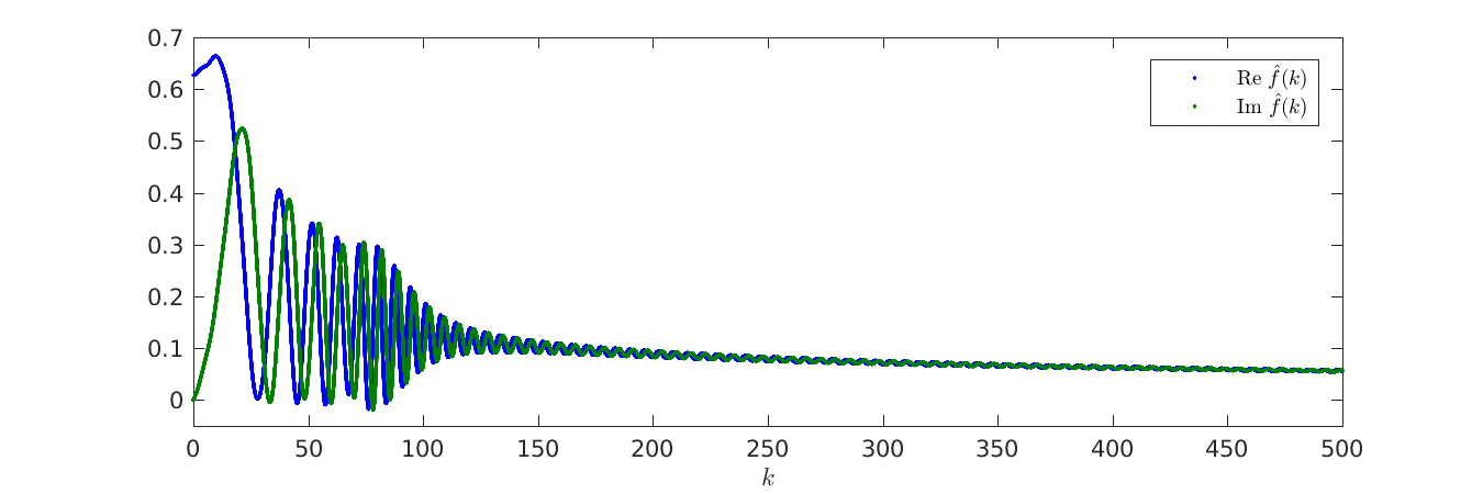
Neither \(f\) nor \(\hat{f}\) is in \(L^2(\mathbb{R})\). Other rules (adaptive, etc) can be designed to efficiently handle various other features of even nastier \(f\) choices.

2D FTs¶

In higher dimensions, the idea is the same: set up a good quadrature rule for your function \(f\), then apply it to the Fourier integral

(2)¶\[\hat{f}({\bf k}) = \int f({\bf x}) e^{i{\bf k}\cdot{\bf x}} d{\bf x} \approx \sum_{j=1}^N f({\bf x}_j) e^{i{\bf k}\cdot{\bf x}_j} w_j\]

for all “target” frequencies \({\bf k}\) in your domain of interest. We demo the case of \(f = \chi_\Omega\), the characteristic function of a bounde domain \(\Omega \subset \mathbb{R}^2\), that is, \(f({\bf x}) = 1\) for \(x\in\Omega\), and \(0\) otherwise. For simplicity, let’s take \(\Omega\) with boundary described in polar coordinates by \(g(\theta) = 1 + 0.3\cos 5\theta\). This enables a simple two-level quadrature scheme, namely an outer \(n\)-node periodic trapezoid rule in \(\theta\), whose integrand is an inner \(m\)-node Gauss-Legendre rule applied to the radial integral. Since \(g\) is smooth, this will have spectral convergence in \(n\) and \(m\). Here is a fresh code to make this quadrature over \(\Omega\):

g = @(t) 1 + 0.3*cos(3*t);                             % boundary shape
n = 280;                                               % # theta nodes
t = 2*pi*(1:n)/n; wt = (2*pi/n);                       % theta nodes, const weights
bx = cos(t).*g(t); by = sin(t).*g(t);                  % boundary points
m = 70;                                                % # r nodes
[xr,wr] = lgwt(m,0,1);                                 % rule for (0,1)
xj = nan(n*m,1); yj = xj; wj = xj;
for i=1:n                                              % loop over angles
  r = g(t(i)); jj = (1:m) + (i-1)*m;                   % this radius; index list
  xj(jj) = cos(t(i))*r*xr; yj(jj) = sin(t(i))*r*xr;    % line of nodes
  wj(jj) = wt*r^2*xr.*wr;            % theta weight times rule for r.dr on (0,r)
end
plot([bx bx(1)],[by by(1)],'-'); hold on; plot(xj,yj,'.');

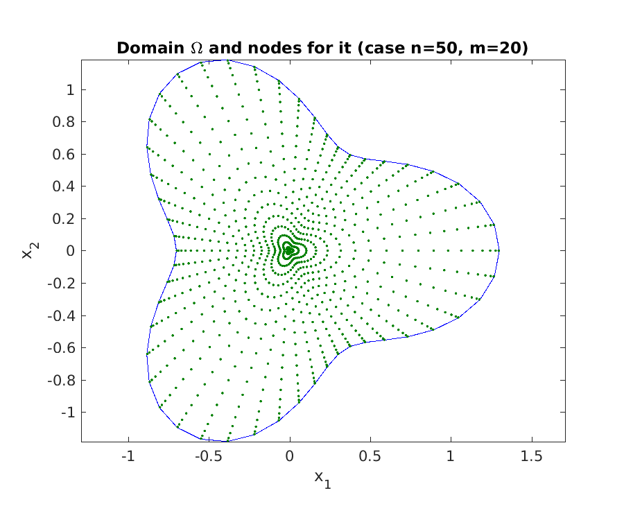
Note that we reduced the numbers of nodes in the plot for clarity. Say we want \(\hat{f}\) on a 2D square grid of frequency targets. We apply the 2D version of the above type 1 scheme. The function is identically 1 in the domain, so the weights simply become the source strengths. We also image the result on a log scale:

kmax = 100;                                            % half the side length in k
M1 = 1e3;                                              % target grid will be M1-by-M1
dk = 2*kmax/M1;
k1 = dk * (-M1/2:(M1/2-1));                            % same 1D freq grid as before
tol = 1e-9;
fhat = finufft2d1(dk*xj, dk*yj, wj, +1, tol, M1, M1);  % M1^2 output nodes
imagesc(k1,k1,log10(abs(fhat))'); axis xy equal tight; colorbar

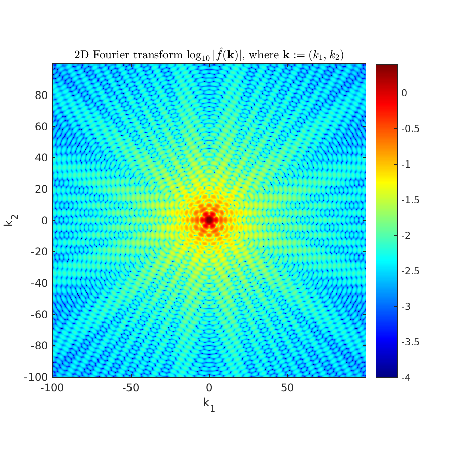
Thus we have computed the 2D FT of a discontinous function on a million-point grid to around 10-digit accuracy in 0.05 sec (the FINUFFT transform time). Note that, as with 1D discontinuous functions, the decay with \(k:=|{\bf k}|\) is slow (it is like \(1/k\)). See the full code tutorial/contft2d.m also for the study that shows that, for the above kmax, convergence to the tolerance has occurred by n=280 and m=70, needing \(N=19600\) nodes. A more efficient set would vary m with \(\theta\).

Note

An application of the above to optics is that \(\Omega\) is a planar scatterer (or its complement, an aperture, via Babinet’s principle) upon which a monochromatic plane wave is incident. The wavelength is small compared to the size of \(\Omega\), so that a scalar Kirchhoff diffraction model is a good one. If a downstream planar detector is very distant (the Fraunhofer diffraction limit), and the angles of scattering are small, then \(|\hat{f}|^2\) is a good model for the detected scattered intensity.

Efficient evaluation of (continuous) Fourier transforms¶

1D FTs evaluated at arbitrary frequencies¶

Faster FTs when frequencies lie on a grid¶

1D FTs of singular functions¶

2D FTs¶

Further reading¶

Table of Contents

Previous topic

Next topic

This Page