Efficient sampling from Gaussian Random Fields (GRFs)
A GRF is a random function defined by its power spectral density (PSD) \(\hat{C}(k)\) as a function of wavevector \(k\). It is thus stationary, ie, its statistical properties are translationally invariant. It is also known as a Gaussian process prior. Given a GRF model, it is important to be able to 1) draw independent samples from the GRF at a given set of target points, and 2) compute the log likelihood (under the model) of a given function values at a given set of target points. We focus on the first application. (For the second, see the Ambikasaran et al reference at the bottom of this page.)
For certain PSDs, independent samples may be generated by solving a PDE with iid random forcing; however this slow and introduces boundary effects. Here we simply use Fourier methods to sample directly from any PSD that is a smooth function of \(k\), and evaluate at arbitrary target points. This is a numerical implementation of the Cramér spectral representation of a GRF (see references below). The idea is that a regular Fourier grid \(k_j\) be used, with spacing sufficiently small based upon the size of the spatial domain in which target points lie. This serves as a good quadrature scheme for any smooth PSD. The GRF model corresponds to random iid coefficients at these Fourier values, with zero mean and variance \(\hat{C}(k_j)\). These coefficients are then evaluated at all target points using a single type 2 NUFFT.
The code is rudimentary but commented to be self-explanatory:
% demo making indep samples from a 1D Gaussian random field, defined by its
% power spectral density \hat{C}(k), using Fourier methods without any BCs.
% Case of NU target pts, hence needs FINUFFT. (Note FFT is ok for unif targs.)
% Barnett 5/24/19
clear

% choose a GRF spectral density function \hat{C}(k)...
form = 'y';   % 'g' is for checking the variance; 'y' is what you care about.
if form=='g'        % Gaussian form (can get superalg convergence wrt K)
  K0 = 2e3;         % freq width, makes smooth below scale 1/K0
  Chat = @(k) (1/sqrt(2*pi)/K0)*exp(-(k/K0).^2/2);
elseif form=='y'    % desired Yukawa form (merely algebraic conv wrt K)
  alpha = 1.0; beta = 100; gamma = 1;    % sqrt(gamma/beta)=0.1 spatial scale
  Chat = @(k) (gamma*k.^2 + beta).^-alpha;
end

% user params...
L = 1;   % we want to evaluate on domain length D=[0,L].
M = 1e4;           % # targs
x = rand(1,M)*L;   % user can choose any target pts
tol = 1e-6;        % desired NUFFT precision
K = 1e4;           % max freq to go out to in Fourier transform for GRF

% alg param setup...
eta = 1.5;         % k-quad scheme convergence param, >=1; maybe =1 is enough?
dk_nyq = pi/L;     % Nyquist k-grid spacing for the width of target domain
dk = dk_nyq/eta;   % k-grid
P = 2*pi/dk        % actual period the NUFFT thinks there is
N = 2*K/dk;        % how many modes, if # k quadr pts.
N = 2*ceil(N/2)    % make even integer
k = (-N/2:N/2-1)*dk;  % the k grid

% check the integral of spectral density (non-stochastic)... 1 for form='g'
I = dk*sum(Chat(k))   % plain trap rule
%figure; loglog(k,Chat(k),'+-'); xlabel('k'); title('check k-quadr scheme');

nr = 3e2;   % # reps, ie indep samples from GRF drawn.. 1e3 takes 3 sec
fprintf('sampling %d times... ',nr);
gvar = zeros(M,1);    % accumulate the ptwise variance
figure;
for r=1:nr
  fk = ((randn(1,N)+1i*randn(1,N))/sqrt(2)) .* sqrt(dk*Chat(k));   % spec ampl
  g = finufft1d2(x/P,+1,tol,fk);                % do it, outputting g at targs
  if r<=5, h=plot(x,real(g),'.'); hold on; end  % show a few samples
  gvar = gvar + abs(g).^2;
end
gvar = gvar/nr;
fprintf('done. mean ptwise var g = %.3f\n',mean(gvar))

xlabel('x'); h2=plot(x,gvar, 'ko'); legend([h h2],'samples g(x)','est var g(x)')
v=axis; v(1:2)=[0 L]; axis(v);
title(sprintf('1D GRF type %s: a few samples, and ptwise variance',form));
The result is as follows, showing 5 samples from a Yukawa or Matern kernel, plus the pointwise variance estimated from 300 samples:
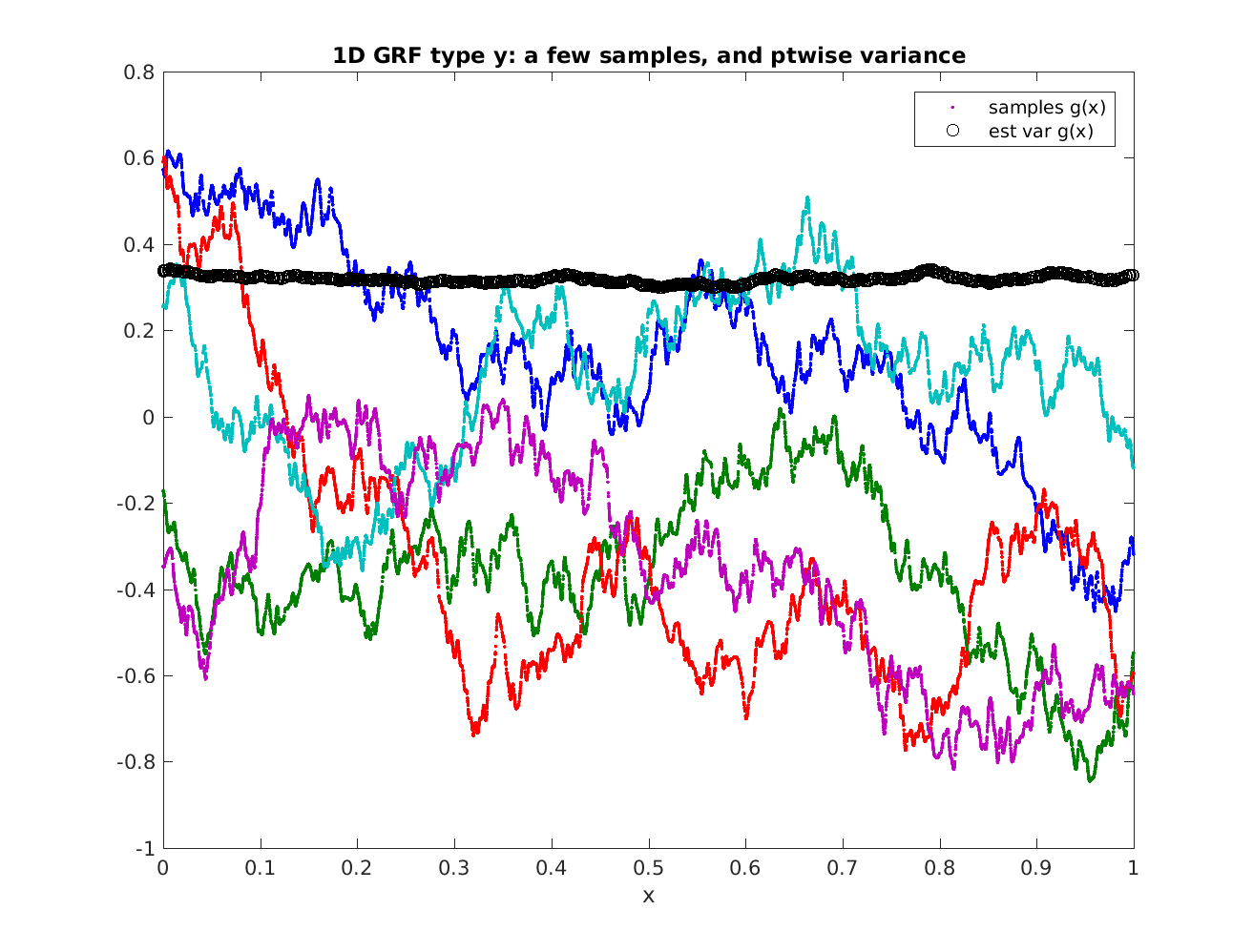
The calculation takes around 1 second.
If \(\hat{C}(k)\) has singularities or discontinuities, a more specialized \(k\)-space quadrature scheme would be preferred for high-order accuracy (low bias). For an example of this, sampling from a 2D GRF, see random plane waves.
Further reading
For background on Gaussian random fields, aka stationary Gaussian processes, see:
C E Rasmussen & C K I Williams, Gaussian Processes for Machine Learning, the MIT Press, 2006. http://www.GaussianProcess.org/gpml
Fast Direct Methods for Gaussian Processes, Sivaram Ambikasaran, Daniel Foreman-Mackey, Leslie Greengard, David W. Hogg, and Michael O’Neil. arxiv:1403.6015 (2015)
For background on computational sampling methods for GRFs (both use crude k-quadrature in the 1D setting):
Shinozuka & Deodatis, “Simulation of Stochastic Processes by Spectral Representation,” Applied Mechanics Reviews 44(4), 191–204 (1991)
On the spectral representation method in simulation, M. Grigoriu, Prob. Engs. Mech. 8(2) 75-80 (1993)